In previous chapters, we covered the fundamentals of PyTorch and applied it to a linear regression example. Now, we will expand on that knowledge by constructing neural networks using PyTorch.
8.1 Modeling Pipeline overview
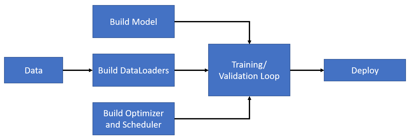
Fig 8.1: Modeling Pipeline in Pytorch
Let’s take a look at the different steps involved in creating a typical modeling pipeline in PyTorch -
Getting the data - PyTorch provides several tools for loading and preprocessing data, such as the torchvision library for image-related tasks or torchtext for natural language processing. You can also create custom data loaders to load data in your desired format.
Build Dataloaders -Once you have your data, you’ll need to create data loaders, which are responsible for batching and shuffling the data during training. Data loaders are essential for efficient training, as they allow you to load and preprocess data in parallel, making use of the GPU capabilities for faster training.
Define Model - Next, you’ll need to define your model architecture. PyTorch provides a wide range of pre-defined layers and modules that you can use to build your neural network. You can also create custom layers or models by subclassing PyTorch’s nn.Module class. Defining your model involves specifying the layers, their connectivity, and any other parameters or hyperparameters that you need for your specific task.
Build Optimizer and Scheduler - Once your model is defined, you’ll need to configure an optimizer and a scheduler. The optimizer is responsible for updating the model’s parameters during training to minimize the loss, while the scheduler adjusts the learning rate to optimize the model’s performance. PyTorch provides various optimization algorithms, such as SGD, Adam, or RMSprop, and scheduling techniques like learning rate decay or cyclical learning rates.
Run training and validation loops - With your data loaders, model, optimizer, and scheduler in place, you’re ready to start the training loop. The training loop typically involves iterating over the data loaders, forwarding the inputs through the model, computing the loss, and backpropagating the gradients to update the model’s parameters. You’ll also need to evaluate your model’s performance on a validation set to monitor its progress during training and avoid overfitting.
Deploy - Once your model has been trained, you can deploy it for inference on new data. PyTorch provides tools for saving and loading model checkpoints, which allows you to reuse your trained model in different applications. You can deploy your model in a variety of environments, such as edge devices, cloud servers, or web applications, depending on your specific requirements.
In summary, a typical modeling pipeline in PyTorch involves getting the data, building data loaders, defining the model architecture, configuring the optimizer and scheduler, implementing the training and validation loop, and finally deploying the trained model for inference in various environments.
Let’s dive into the practical implementation of a modeling pipeline in PyTorch using the popular MNISTdataset as an example. We’ll follow the steps outlined above to build our first neural network from scratch.
8.2 Downloading Data from Kaggle
The dataset we will be utilizing is the MNIST png dataset from Kaggle, as opposed to the CSV version, for a more practical experience.
Here are few steps you need to perform before we download the data -
If you don’t have a Kaggle account, you can make one for free here.
To download the dataset, you will need kaggle installed, you can run the following command in notebook or CLI.
!pip install kaggle >> /dev/null
Have a kaggle.json stored in ~/.kaggle. You can get your token by going to Your Profile -> Account -> Create New API Token.
Once you have the above three steps done, run the API command provided:
To examine the file system, we will utilize the fastcorePath function. It enhances the functionality of python’s Path class and simplifies the process of inspecting directories and folders.
from fastcore.xtras import Pathzip_path = Path("../data/mnist-png.zip")zip_path.exists() # Check if the file exist
True
The data has been persisted to the mnist-png.zip file on the local system, within the ../data directory. The next step is to utilize the zipfile package to extract the contents of the archive.
Warning
The execution of the following code block will take a significant amount of time(6-10 mins) as it involves the extraction of 70,000 PNG images.
# Output directorydPath = Path("../data/")# Unzipping data file in output directoryimport zipfilewith zipfile.ZipFile(zip_path, "r") as zip_ref: zip_ref.extractall(str(dPath))# Removing the original zip filezip_path.unlink()# Removing duplicate folder in the unzipped dataimport shutildPath = dPath/'mnist_png'shutil.rmtree(dPath/'mnist_png')
Each of these digit subfolders contains images. We will proceed to load a few of these images.
from PIL import Imagefrom IPython.display import displayfor img in [Image.open((dPath/'training/0').ls()[0]), Image.open((dPath/'training/1').ls()[0]), Image.open((dPath/'training/2').ls()[0]), Image.open((dPath/'training/3').ls()[0])]: display(img)
8.3 Creating Dataset Object
As previously discussed, prior to training the model, it is necessary to establish a data pipeline in PyTorch. This includes defining a Dataset object and subsequently loading it via a PyTorch Dataloader.
8.3.1 Using Pure Pytorch
Initially, we will demonstrate the process of constructing a custom image Dataset object using pure PyTorch. To begin, we will import the necessary libraries.
By utilizing glob, we have successfully obtained the filepaths of all images within the training and testing folders. We can see there are 60,000 training images and 10,000 testing images. The next step is to extract the labels from the folder names.
As we can see above, ImageDataset is a custom PyTorch Dataset class. Let’s walk through the components -
The class takes two inputs in its constructor, X and y, which are lists of image file paths and corresponding labels respectively. These are stored as class variables self.img_paths and self.targets.
The __len__ method returns the number of images in the dataset by returning the length of self.img_paths list.
The __getitem__ method is called when a specific sample is requested from the dataset. It takes an index as an argument, and returns a tuple of the image data and the corresponding label for that index. The image is processed as follows -
It opens the image file at the index passed in the argument using PIL(Python Imaging Library) Image.open function
Converts it to a numpy array
Flattens it (convert it from 28x28 2d array to 784 1-d array)
Normalizes it by dividing by 255 floating number
We will now proceed to instantiate our ImageDataset class for both thetraining and testing datasets
One object: Image Tensor of shape torch.Size([784]), Label: 0
One object: Image Tensor of shape torch.Size([784]), Label: 3
8.3.2 Using Torchvision
We have demonstrated the procedure of creating a custom ImageDataset object. Now we will examine how to simplify this process by utilizing the torchvision package. The torchvision package encompasses commonly used datasets, model architectures, and image transformations for computer vision tasks.
To begin, we will import the datasets and transforms modules from the torchvision package.
from torchvision import datasetsfrom torchvision import transformsfrom tqdm.auto import tqdm
Next we will use datasets and transform modules to load our MNIST images.
Length of train dataset: 60000, test_dataset: 10000
One object: Image Tensor of shape torch.Size([784]), Label: 0
Let’s look at the code above:
The first step is to define a transform object using the transforms.Compose function. This function takes a list of transformation functions as an argument and applies them in the order they are passed in. In this case, the following transformations are applied:
transforms.Grayscale(): Convert the images to grayscale
transforms.ToTensor(): Converts the images to PyTorch tensors
transforms.Lambda(lambda x: torch.flatten(x)): Flatten the tensors from 28x28 2-D arrayto 784 1-D array
Next, it creates two datasets for training and testing using the datasets.ImageFolder class. It takes the root directory of the dataset and the transform object as the arguments. It automatically creates a label for each image by taking the name of the folder where the image is stored.
The code then prints the length of the train and test datasets and the shape and label of the first object in the train dataset. The datasets.ImageFolder class is a convenient way to create a Pytorch dataset from a directory of images and it is useful when you have the data in a structured way.
8.4 Create a Dataloader
Create a dataloader using torch.utils.data.DataLoader function.
The torch.utils.data.DataLoader class takes a dataset object as an argument and returns an iterator over the dataset object. It can be used to load the data in batches, shuffle the data, and apply other useful functionality.
In the above code, following parameters are passed to the DataLoader:
train_ds and test_ds are the training and testing datasets respectively.
batch_size=128: The number of samples per batch.
shuffle=True for the training dataset, and shuffle=False for the testing dataset: whether to shuffle the data before iterating through it.
num_workers=num_workers: the number of worker threads to use for loading the data. Here it is set to half of the number of CPU cores using os.cpu_count() method.
It returns two data loaders, one for the training dataset and one for the testing dataset. The data loaders can be used as iterators to access the data in batches. This allows to load the data in smaller chunks, making it more memory efficient and faster to train.
As we can observe, each batch comprises of an input tensor of shape (128x784) representing 128 images of flattened (28x28) dimension, and a label tensor of shape (128) representing the corresponding digit labels for the images.
8.5 Defining our Training and Validation loops
We will now implement the training loop. It is similar to the training loop we constructed in chapter 6.
## Training loopdef train_one_epoch(model, data_loader, optimizer, loss_func): total_loss, nums =0, 0for batch in tqdm(iter(data_loader)):## Taking one mini-batch xb, yb = batch[0].to(dev), batch[1].to(dev) y_pred = model.forward(xb)## Calculation mean square error per min-batch nums +=len(yb) loss = loss_func(y_pred, yb) total_loss += loss.item() *len(yb)## Computing gradients per mini-batch loss.backward()## Update model parameters and zero grad optimizer.step() optimizer.zero_grad()return total_loss / nums
The train_one_epoch function takes 4 arguments:
model: The model to be trained
data_loader: The data loader for the training dataset
optimizer: The optimizer used to update the model parameters
loss_func: The loss function used to calculate the error of the model
The function uses a for loop to iterate through the data loader. For each mini-batch of data, it performs the following steps:
It loads the data and the labels from the data loader and sends it to the device.
It makes a forward pass through the model to get the predictions and then calculates the loss using the loss function.
It computes the gradients of the model parameters with respect to the loss.
It updates the model parameters using the optimizer and zero the gradients.
The total_loss and nums variables are used to keep track of the total loss and number of samples seen during the epoch.
The code above defines an MLP model as a Pytorch nn.Module class. The class takes in two arguments, n_in and n_out which represents the number of input features and the number of output features of the model respectively. The class is a simple Multi-layer Perceptron model with 3 hidden layers. Each hidden layer have a linear layer with a ReLU activation function. The forward method takes in input tensor x and returns the output by passing it through the defined sequential model.
Let’s define our training parameters.
dev = torch.device("cuda") if torch.cuda.is_available() else torch.device("cpu")loss_func = nn.CrossEntropyLoss()model = MLP(784,10).to(dev)optimizer = torch.optim.SGD(model.parameters(), lr=1e-3)epochs =5
This code is preparing the model, loss function, optimizer, and the number of training epochs to train the MLP model.
dev = torch.device("cuda") if torch.cuda.is_available() else torch.device("cpu"): This line of code is determining which device to use for training. If a CUDA-enabled GPU is available, the model and data will be moved to the GPU for faster training, otherwise it will use the CPU.
loss_func = nn.CrossEntropyLoss(): This line of code is defining the loss function for the model. CrossEntropyLoss is a commonly used loss function for multi-class classification problems.
model = MLP(784,10).to(dev): This line of code is instantiating the MLP model with 784 input features and 10 output features, and then moving it to the device.
optimizer = torch.optim.SGD(model.parameters(), lr=1e-3): This line of code is creating an optimizer with Stochastic Gradient Descent (SGD) algorithm and a learning rate of 1e-3. The optimizer updates the model parameters during training to minimize the loss function.
epochs = 5: This line of code is specifying the number of training epochs. An epoch is one complete pass through the entire training dataset.
We will now evaluate the performance of our model on the validation dataset before training.
test_loss, test_acc = validate_one_epoch(model=model, data_loader=test_dls, loss_func=loss_func)print(f"Random model: Test Loss: {test_loss:.4f}, Test Accuracy: {test_acc:.4f}")
Random model: Test Loss: 2.3025, Test Accuracy: 0.0772
As anticipated, the model’s accuracy is low, around 7-8%, due to the fact that it has not been trained yet.
We will now encapsulate our previously defined functions in a fit function, which will be responsible for both training and evaluating the model.
Epoch 1,Train Loss: 0.3480, Test Loss: 0.1660, Valid Accuracy: 0.9501
Epoch 2,Train Loss: 0.1392, Test Loss: 0.1289, Valid Accuracy: 0.9597
Epoch 3,Train Loss: 0.0895, Test Loss: 0.0931, Valid Accuracy: 0.9699
Epoch 4,Train Loss: 0.0659, Test Loss: 0.0758, Valid Accuracy: 0.9759
Epoch 5,Train Loss: 0.0490, Test Loss: 0.0700, Valid Accuracy: 0.9797
By utilizing the AdamW optimizer and MLP model, we can see that after 5 epochs, we have a highly accurate model with a 98% accuracy as compared to random prediction of 7-8%.
8.7 Training using a simple CNN model
As previously demonstrated, the fit function is highly adaptable as we were able to change our optimizer without making any modifications to the function. Now, we will replace our MLP model with a CNN (Convolutional Neural Network) model. We will begin by defining a basic CNN network.
The code above defines a class called Mnist_CNN which is a subclass of nn.Module. It creates an object of the class and initiates three 2D convolutional layers(conv1, conv2, conv3) with different input and output channels, kernel size, stride and padding. The forward method applies the convolution operation on the input tensor with relu activation function, then average pooling is applied to the output tensor and the final output tensor is reshaped to a 1-D tensor.
Now, we can pass an instance of this model to the fit function for training and validation.
Epoch 1,Train Loss: 1.8228, Test Loss: 1.4976, Valid Accuracy: 0.5442
Epoch 2,Train Loss: 1.3562, Test Loss: 1.2602, Valid Accuracy: 0.5958
Epoch 3,Train Loss: 1.2113, Test Loss: 1.1522, Valid Accuracy: 0.6144
Epoch 4,Train Loss: 1.1286, Test Loss: 1.0886, Valid Accuracy: 0.6187
Epoch 5,Train Loss: 1.0741, Test Loss: 1.0454, Valid Accuracy: 0.6308
As can be observed, we are able to seamlessly switch from an MLP to a CNN model by utilizing the adaptable fit function and train the model.
8.8 Conclusion
In this chapter, we progressed from a basic linear regression example to building an image classifier using MLP and CNN models. We gained practical experience in creating custom Dataset and Dataloader objects and were introduced to the torchvision library for simplifying this process. Additionally, we developed a versatile fit function, which can be utilized with various models, optimizers, and loss functions for training our models.
The idea of flexibility as demonstrated in the fit function is not unique, and there are many frameworks that aim to simplify the model training process by offering high-level APIs, allowing machine learning scientists to focus on building and solving problems, while the frameworks handle the majority of the complexity. Later in the book, we will repeat the same exercise using the fastai library, which is a highly flexible and performant framework built on top of PyTorch, and observe how we can construct neural networks with minimal lines of code.