Code
import numpy as np
from collections import CounterPart 3 of the diversity series: Why one-size-fits-all diversity doesn’t work, and how to personalize it per user.
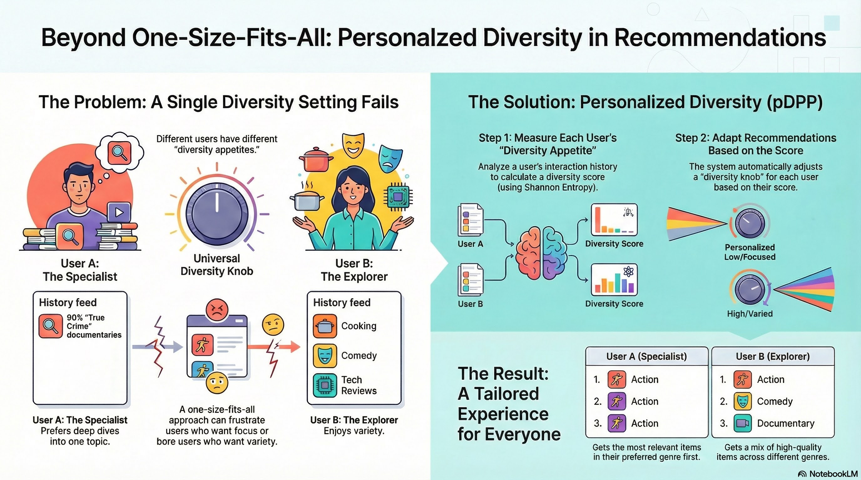
In Part 2, we explored how DPP balances relevance and diversity using a single parameter α. But there’s a catch: we used the same α for every user.
Think about it. On a video platform like YouTube or Reels, you’ll find:
Should we show both users the same amount of diversity? Probably not.
User A has a clear, focused preference. Pushing diverse content might feel random or irrelevant to them. User B, on the other hand, has shown they enjoy variety. A narrowly focused feed might bore them.
This is the core limitation of standard DPP: it treats diversity as a system-level knob, not a user-level preference. The solution? Personalized DPP (pDPP), which adapts the diversity-relevance tradeoff per user based on their historical behavior.
The idea comes from a Huawei research paper on personalized re-ranking, and the implementation is surprisingly simple: we measure how “diverse” each user’s past interactions have been using information theory (Shannon entropy), then use that to personalize α.
In this post, we’ll:
Let’s get into it.
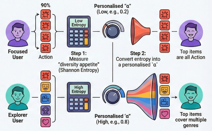
How do we measure a user’s appetite for diversity? The Huawei paper uses Shannon entropy over the user’s interaction history.
Shannon entropy measures the “surprise” or “spread” in a distribution. If a user watches videos from 10 genres equally, entropy is high (maximum uncertainty about what they’ll watch next). If they watch 95% from one genre, entropy is low (very predictable).
This gives us a principled, interpretable metric: we’re not guessing what users want; we’re measuring what they’ve demonstrated through their actions.
| User Type | Interaction Pattern | Entropy | Diversity Preference |
|---|---|---|---|
| Focused (User A) | 90% one genre | Low | Prefers less diversity |
| Explorer (User B) | Spread across genres | High | Prefers more diversity |
The next step is to turn this entropy score into a personalized α value. A user with high entropy gets a higher α (more diversity weight), while a user with low entropy gets a lower α (more relevance weight).
Let’s formalize the intuition from the previous section. For a user u, we compute Shannon entropy over their genre distribution:
H(u) = -Σ P(g|u) × log(P(g|u))
Where:
P(g|u) is the probability of genre g in user u’s interaction historyLet’s implement this:
import numpy as np
from collections import Counterdef compute_entropy(genre_list: list[str]) -> float:
"""Compute Shannon entropy over a list of genre interactions."""
if not genre_list: return 0.0
genre_counts = Counter(genre_list)
total = len(genre_list)
entropy = 0.0
for count in genre_counts.values():
p = count / total
entropy -= p * np.log(p)
return entropy
# User A: watches mostly one genre (narrow taste)
user_a_genres = ['action', 'action', 'action', 'action', 'comedy']
# User B: watches many genres (diverse taste)
user_b_genres = ['action', 'comedy', 'drama', 'documentary', 'horror']
print(f"User A(narrow taste) entropy: {compute_entropy(user_a_genres):.3f}")
print(f"User B(diverse taste) entropy: {compute_entropy(user_b_genres):.3f}")User A(narrow taste) entropy: 0.500
User B(diverse taste) entropy: 1.609The numbers confirm our intuition:
User A (entropy = 0.500): With 4 action + 1 comedy, their behavior is highly predictable. Low entropy means low “surprise” in what they’ll watch next.
User B (entropy = 1.609): With equal spread across 5 genres, their behavior is maximally uncertain. This is actually the maximum possible entropy for 5 categories: ln(5) ≈ 1.609.
What the values mean practically:
So User B’s entropy being exactly log(5) tells us they have a perfectly uniform distribution across genres. User A’s 0.500 is much closer to 0, reflecting their strong single-genre preference.
This entropy value becomes our “diversity propensity score” that we’ll use to personalize α in the next section.
Now we have each user’s entropy score. How do we turn it into a personalized α?
Huawei paper uses a simple multiplicative formula:
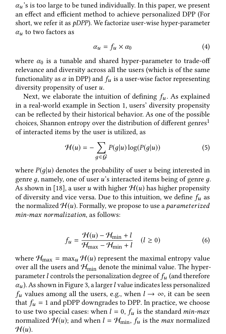
α_u = f_u × α_0
Where:
α_0 is your baseline diversity weight (the system default)f_u is a user-specific scaling factor between 0 and 1The scaling factor f_u is computed via min-max normalization of the user’s entropy:
f_u = (H_u - H_min + l) / (H_max - H_min + l)
Where:
H_u is the user’s entropyH_min, H_max are the min/max entropy across your user populationl is a smoothing parameterThe l parameter as a personalization dial:
l = 0: Full personalization. Users at H_max get f_u = 1, users at H_min get f_u = 0l → ∞: No personalization. Everyone gets f_u ≈ 0, so α_u ≈ 0 for all usersl in the range of H_max - H_min gives moderate personalizationLet’s implement it:
def compute_f_u(H_u, H_min, H_max, l=0):
    return (H_u - H_min + l) / (H_max - H_min + l)
# Show how l controls personalization strength
print("Effect of smoothing parameter l on f_u:")
print("-" * 50)
print(f"{'l':<10} {'User A f_u':<15} {'User B f_u':<15} {'Difference':<10}")
print("-" * 50)
H_a = compute_entropy(user_a_genres) # ~0.5
H_b = compute_entropy(user_b_genres) # ~1.609
# For this example, assume population-wide bounds
H_min, H_max = 0.5, 1.61 # You'd compute these from your user base
for l in [0, 0.25, 0.5, 1.0, 2.0]:
f_a = compute_f_u(H_a, H_min, H_max, l)
f_b = compute_f_u(H_b, H_min, H_max, l)
print(f"{l:<10} {f_a:<15.3f} {f_b:<15.3f} {f_b - f_a:<10.3f}")Effect of smoothing parameter l on f_u:
--------------------------------------------------
l User A f_u User B f_u Difference
--------------------------------------------------
0 0.000 0.999 0.999
0.25 0.184 1.000 0.815
0.5 0.311 1.000 0.689
1.0 0.474 1.000 0.526
2.0 0.643 1.000 0.357 As l increases, the gap between User A and User B shrinks. At l=0, we get maximum personalization (f_u ranges from 0 to 1). At l=2, both users are clustered around 0.5, meaning they get nearly the same diversity treatment. This lets you tune how aggressively the system personalizes: start conservative with higher l, then decrease it as you gain confidence in the entropy signal.
Now let’s bring in our DPP functions from Part 2.
def greedy_map_dpp(L, k):
    N = L.shape[0]
    selected = []
    remaining = set(range(N))

    for _ in range(k):
        best_item, best_det = None, -1

        for item in remaining:
            candidate_set = selected + [item]
            det_val = np.linalg.det(L[np.ix_(candidate_set, candidate_set)])

            if det_val > best_det:

                best_det = det_val
                best_item = item

        selected.append(best_item)
        remaining.remove(best_item)

    return selected

def youtube_dpp_kernel(relevance, embeddings, alpha=0.5, sigma=1.0):
    N = len(relevance)
    L = np.zeros((N, N))

    # Compute pairwise distances
    # D_ij = ||embedding_i - embedding_j||²
    for i in range(N):
        for j in range(N):
            if i == j:
                # Diagonal: quality squared

                L[i, i] = relevance[i] ** 2
            else:
                # Off-diagonal: scaled similarity with RBF kernel
                D_ij = np.sum((embeddings[i] - embeddings[j]) ** 2)
                similarity = np.exp(-D_ij / (2 * sigma**2))
                L[i, j] = alpha * relevance[i] * relevance[j] * similarity

    return L

def youtube_dpp_ranking(relevance, embeddings, k, alpha=0.5, sigma=1.0):
    W = list(range(len(relevance)))  # Remaining candidate indices
    R = []  # Final ranked list

    while len(W) > 0:
        # Build kernel for current candidate pool
        rel_W = relevance[W]
        emb_W = embeddings[W]
        L = youtube_dpp_kernel(rel_W, emb_W, alpha=alpha, sigma=sigma)

        # Select up to k items from current pool
        window_size = min(k, len(W))
        M = greedy_map_dpp(L, k=window_size)

        # Map back to original indices
        selected_items = [W[i] for i in M]
        R.extend(selected_items)

        # Remove selected items from candidate pool
        W = [w for w in W if w not in selected_items]

    return R
Let’s create the personalized version.
def compute_user_alpha(genre_history, H_min, H_max, alpha_0, l=0):
    """Compute personalized alpha for a user based on their genre history."""
    H_u = compute_entropy(genre_history)
    f_u = compute_f_u(H_u, H_min, H_max, l)
    return f_u * alpha_0

def pdpp_ranking(relevance, embeddings, k, genre_history, H_min, H_max, alpha_0=1.0, l=0, sigma=1.0):
    """Personalized DPP ranking using user's genre history."""
    alpha_u = compute_user_alpha(genre_history, H_min, H_max, alpha_0, l)
    print(f"User alpha: {alpha_u:.4f} (base alpha_0={alpha_0})")
    return youtube_dpp_ranking(relevance, embeddings, k, alpha=alpha_u, sigma=sigma)

# 5 videos with relevance scores and genre embeddings (2D for simplicity)
relevance = np.array([0.9, 0.85, 0.8, 0.7, 0.6, 0.5])
genre = ['Action', 'Action', 'Action', 'Comedy', 'Documentary', 'Mixed comedy/documentary']

# Embeddings: action movies are close together, others spread out
embeddings = np.array([
    [1.0, 0.0, 0.0],   # video 0: pure action
    [0.9, 0.1, 0.0],   # video 1: action (very similar to 0)
    [0.8, 0.1, 0.1],   # video 2: action (also very similar to 0)
    [0.0, 1.0, 0.0],   # video 3: comedy
    [0.0, 0.0, 1.0],   # video 4: documentary
    [0.1, 0.5, 0.5],   # video 5: mixed
])

# Global entropy bounds (you'd compute these from your user population)
H_min, H_max = 0.5, 1.61

# Compare rankings for User A (narrow taste) vs User B (diverse taste)
print("=== User A (narrow taste - prefers action) ===")
ranking_a = pdpp_ranking(relevance, embeddings, k=6, genre_history=user_a_genres, H_min=H_min, H_max=H_max, l=0)
print(f"Top 6: {[genre[i]+'('+str(relevance[i])+')' for i in ranking_a[:6]]}")

print("=== User B (diverse taste) ===")
ranking_b = pdpp_ranking(relevance, embeddings, k=6, genre_history=user_b_genres, H_min=H_min, H_max=H_max, l=0)
print(f"Top 6: {[genre[i]+'('+str(relevance[i])+')' for i in ranking_b[:6]]}")
=== User A (narrow taste - prefers action) ===
User alpha: 0.0004 (base alpha_0=1.0)
Top 6: ['Action(0.9)', 'Action(0.85)', 'Action(0.8)', 'Comedy(0.7)', 'Documentary(0.6)', 'Mixed comedy/documentary(0.5)']
=== User B (diverse taste) ===
User alpha: 0.9995 (base alpha_0=1.0)
Top 6: ['Action(0.9)', 'Comedy(0.7)', 'Documentary(0.6)', 'Mixed comedy/documentary(0.5)', 'Action(0.8)', 'Action(0.85)']The results show exactly what we’d expect:
User A (α ≈ 0.0) gets the three action movies upfront, ranked purely by relevance. With α near zero, diversity has almost no influence. The algorithm respects their focused history: “You’ve watched action 80% of the time, so here’s the best action content first.”
User B (α ≈ 1.0) sees a completely different pattern. They get one action movie, then the algorithm immediately jumps to comedy, documentary, and mixed content. The other two action movies get pushed to positions 5 and 6. Their high entropy history translates to high α, which penalizes clustering similar items together.
Same 6 videos. Same relevance scores. Completely different experiences.
This is the power of pDPP: rather than treating diversity as a global system setting, it becomes a per-user preference learned directly from behavior. User A’s narrow feed isn’t a bug; it’s what their history tells us they want. User B’s varied feed isn’t random; it matches their demonstrated exploration pattern.
The multiplicative formula α_u = f_u × α_0 has a problem: it can be too aggressive. Look at User A’s result above: with f_u ≈ 0, they got α ≈ 0, meaning zero diversity consideration. In production, you probably don’t want to completely eliminate diversity for anyone.
The multiplicative approach also lacks intuitive bounds. If your team decides “we never want α below 0.4 or above 0.8,” the multiplicative formula doesn’t give you that control directly.
The additive bounded formulation:
Instead of multiplying, we use an additive offset centered around 0.5:
α_u = α_0 + (f_u - 0.5) × α_range
Where:
α_0 is your baseline (center point)α_range controls how far users can deviate from baselinef_u - 0.5 shifts the range to [-0.5, +0.5], so the adjustment is symmetricThis gives you explicit floor and ceiling:
α_0 - 0.5 × α_rangeα_0 + 0.5 × α_rangeFor example, with α_0 = 0.6 and α_range = 0.4:
α = 0.6 - 0.2 = 0.4 (most focused users)α = 0.6 + 0.2 = 0.8 (most diverse users)def compute_user_alpha_bounded(genre_history, H_min, H_max, alpha_0=0.6, alpha_range=0.4, l=0):
"""Compute personalized alpha with explicit floor/ceiling bounds."""
H_u = compute_entropy(genre_history)
f_u = compute_f_u(H_u, H_min, H_max, l)
# Additive formulation: center at alpha_0, vary by alpha_range
alpha_u = alpha_0 + (f_u - 0.5) * alpha_range
return alpha_u
def pdpp_ranking_bounded(relevance, embeddings, k, genre_history, H_min, H_max,
alpha_0=0.6, alpha_range=0.4, l=0, sigma=1.0):
"""Personalized DPP with bounded additive alpha."""
alpha_u = compute_user_alpha_bounded(genre_history, H_min, H_max, alpha_0, alpha_range, l)
return youtube_dpp_ranking(relevance, embeddings, k, alpha=alpha_u, sigma=sigma)
print("=== User A (narrow taste) - Bounded ===")
ranking_a_bounded = pdpp_ranking_bounded(
relevance, embeddings, k=6, genre_history=user_a_genres,
H_min=H_min, H_max=H_max, alpha_0=0.6, alpha_range=0.4
)
print(f"Top 6: {[genre[i]+'('+str(relevance[i])+')' for i in ranking_a_bounded]}\n")
print("=== User B (diverse taste) - Bounded ===")
ranking_b_bounded = pdpp_ranking_bounded(
relevance, embeddings, k=6, genre_history=user_b_genres,
H_min=H_min, H_max=H_max, alpha_0=0.6, alpha_range=0.4
)
print(f"Top 6: {[genre[i]+'('+str(relevance[i])+')' for i in ranking_b_bounded]}")=== User A (narrow taste) - Bounded ===
Top 6: ['Action(0.9)', 'Action(0.85)', 'Action(0.8)', 'Comedy(0.7)', 'Documentary(0.6)', 'Mixed comedy/documentary(0.5)']
=== User B (diverse taste) - Bounded ===
Top 6: ['Action(0.9)', 'Comedy(0.7)', 'Documentary(0.6)', 'Action(0.85)', 'Action(0.8)', 'Mixed comedy/documentary(0.5)']Now both users stay within the guardrails we set (0.4 to 0.8):
User A (α = 0.4) still gets all three action movies first, but now there’s some diversity consideration baked in. They’re at the floor, not at zero. If we had more videos in the candidate pool, this baseline diversity would prevent completely homogeneous results.
User B (α = 0.8) gets a diversified feed, but not as extreme as before. Compare to the multiplicative version where they had α ≈ 1.0: now the second action movie appears at position 4 instead of position 5. The ceiling prevents over-diversification.
Why this matters in production:
The tradeoff is less dramatic personalization. The multiplicative approach gave a 10x difference between User A and B (0.0 vs 1.0). The bounded approach gives a 2x difference (0.4 vs 0.8). Which is right depends on your product goals and risk tolerance.
Deploying pDPP requires a few decisions that don’t show up in toy examples.
Computing H_min and H_max
You need population-wide entropy bounds. Two approaches:
Batch computation: Run a daily/weekly job over all active users, compute their entropy, store the min/max. Simple, but lags behind distribution shifts.
Approximate with theory: If you have n genres, the theoretical bounds are H_min = 0 (user watches one genre) and H_max = ln(n) (uniform distribution). This avoids the batch job but may not reflect your actual user distribution.
In practice, I’d recommend starting with theoretical bounds, then validating against your actual user distribution. If 99% of users fall between 0.3 and 1.2 but your theoretical max is 2.3, you’re wasting personalization range.
Cold Start
New users have no history, so no entropy. Options:
α_0 (the baseline) until they have N interactionsHow Often to Update f_u
Entropy is relatively stable for established users. Someone who’s watched 500 videos won’t see their entropy swing wildly from one more view. Options:
For most systems, daily batch is sufficient. Entropy changes slowly.
What Counts as “Genre”?
The paper uses genre, but you can use any categorical attribute:
You can even combine multiple: compute entropy over (genre, creator_type) tuples. The key is choosing attributes that meaningfully capture “diversity” for your product.
Standard DPP’s single α ignores that users have different diversity appetites. Shannon entropy over interaction history gives us a principled way to measure each user’s diversity propensity from their behavior.
pDPP personalizes the relevance-diversity tradeoff per user. High-entropy users (explorers) get more diversity; low-entropy users (focused) get more relevance.
The bounded additive formulation is production-friendly. It gives explicit floor/ceiling control and prevents edge cases where diversity is completely eliminated.
Previous posts in this series:
I hope this series has been useful for thinking about diversity in your recommendation systems! If you’re experimenting with pDPP or have questions, connect with me on LinkedIn to share your experience.