Mixing art into the science of model explainability

Explainability
Machine Learning
Author

Aayush Agrawal

Published

September 23, 2022

Overview on Explainable Boosting Machine and an approach for converting ML explanation to more human-friendly explanation.

Fig.1 - A lego figure on my desk

1. Science of ML explainability

1.1 The Interpretability vs Accuracy Trade-off

In traditional tabular machine learning approaches, Data scientists often deal with the trade-off b/w interpretability and accuracy.

Fig.2: Interpretability/Intelligibility and Accuracy Tradeoff
Image Credit - The Science Behind InterpretML: Explainable Boosting Machine

As shown in the chart above, we can see that Glass-Box models like Logistic Regression, Naive Bayes, and Decision Trees are simple models to interpret, and predictions from these models are not highly accurate. On the other hand, Black-Box models like Boosted Trees, Random Forest, and Neural Nets are hard to interpret but lead to highly accurate predictions.

1.2 Introducing EBMs

To solve the problem just mentioned above EBMs(Explainable Boosted Machine) model was developed by Microsoft Research1. “Explainable Boosting Machine (EBM) is a tree-based, cyclic gradient boosting Generalized Additive Model with automatic interaction detection. EBMs are often as accurate as state-of-the-art BlackBox models while remaining completely interpretable. Although EBMs are often slower to train than other modern algorithms, EBMs are extremely compact and fast at prediction time.”2

Fig.3: EBMs breaking the Interpretability vs Accuracy paradox
Image Credit - The Science Behind InterpretML: Explainable Boosting Machine

As we can see from the chart above, EBMs help us break out of this trade-off paradox and help us build models which are both highly interpretable and accurate. To further understand the math behind EBMs I highly encourage watching this 12-minute YouTube video -

Video - The Science Behind InterpretML: Explainable Boosting Machine

1.3 Glass box vs Black box models. What to choose?

Tip

The answer to every complex question in life is “It depends”.

There are trade-offs b/w using Glassbox models as compared to Blackbox models. There is no clear winner in picking one model over the other but depending on the situation DS can make an educated guess on what model to pick.

Fig.4: Glassbox models vs BlackBox models

Two considerations to think about while picking glass box vs black box models are the following-

1) Explainability Requirements - In the domain where there is no need for explanation or it is needed for a data scientist or technical audience for intuition/inspection purposes, in these cases, DS are well off using black box models. In the domain where an explanation is needed because of business or regulatory requirements or where these explanations are served to a non-technical audience (humans), glass-box models have an upper hand. This is because explanations coming out of the glass box models are exact and global.

Note

Exact and global just means that a value of a particular feature will always have the same effect on each prediction explanation. For example, in the case of the prediction of income of a particular individual being above $50k with age as one of the predictors, if the age is 40 and it will impact the target variable with the same proportion let us say 5% in each observation in the data where the age is 40. This is not the case when we build explanations through LIME and Shapely for black box models. In black-box models, age with the value 40 for example can have a 10% lift in an individual probability of their income being above 50k for one observation and -10% lift in the other.

2) Compute Requirement - DS needs to pay attention to various compute requirements for testing and training a model depending on its use case. EBMs are particularly slow in the training phase but provide fast predictions with built-in explanations. So, in cases where you need to train your model every hour, EBMs might not suffice your need. But, in cases where the training of the model happens monthly/weekly, and scores are generated on a more frequent basis (hourly/daily) EBMs might fit the use case well. Also, in cases where you might be required to produce an explanation for each prediction EBMs can save a lot of computing and might be the only feasible technique to use for millions of observations. Look below to understand the operational difference b/w EBMs and other tree-based ensemble methods.

Fig. 5: EBMs vs XgBoost/LightGBM

2. Hands on with EBMs

2.1 Data Overview

For this example, we will use Adult Income Dataset from the UCI machine learning Repository3. The problem in this dataset is set up as a binary classification problem to predict if a certain individual income based on various census information (education level, age, gender, occupation, etc.) exceeds $50K/year. For sake of simplicity, we are only going to use observations of individuals in the United States and the following predictors -

  • Age: continuous variable, individuals’ age
  • Occupation: categorical variable, Tech-support, Craft-repair, Other-service, Sales, Exec-managerial, Prof-specialty, Handlers-cleaners, Machine-op-inspct, Adm-clerical, Farming-fishing, Transport-moving, Priv-house-serv, Protective-serv, Armed-Forces.
  • HoursPerWeek: continuous variable, amount of hours spent in a job per week
  • Education: categorical variable, Bachelors, Some-college, 11th, HS-grad, Prof-school, Assoc-acdm, Assoc-voc, 9th, 7th-8th, 12th, Masters, 1st-4th, 10th, Doctorate, 5th-6th, Preschool.
Code
## Importing required libraries
import pandas as pd
import numpy as np
from sklearn.model_selection import train_test_split
from sklearn import metrics
from interpret.glassbox import ExplainableBoostingClassifier
from interpret import show
import warnings
import plotly.io as pio
import plotly.express as px
warnings.filterwarnings('ignore')
pio.renderers.default = "plotly_mimetype+notebook_connected"
## Loading the data
df = pd.read_csv( "https://archive.ics.uci.edu/ml/machine-learning-databases/adult/adult.data", header=None)
df.columns = [
    "Age", "WorkClass", "fnlwgt", "Education", "EducationNum",
    "MaritalStatus", "Occupation", "Relationship", "Race", "Gender",
    "CapitalGain", "CapitalLoss", "HoursPerWeek", "NativeCountry", "Income"
]

## Filtering for Unites states
df = df.loc[df.NativeCountry == ' United-States',:]

## Only - Taking required columns
df = df.loc[:,["Education", "Age","Occupation", "HoursPerWeek", "Income"]]

df.head()
Education Age Occupation HoursPerWeek Income
0 Bachelors 39 Adm-clerical 40 <=50K
1 Bachelors 50 Exec-managerial 13 <=50K
2 HS-grad 38 Handlers-cleaners 40 <=50K
3 11th 53 Handlers-cleaners 40 <=50K
5 Masters 37 Exec-managerial 40 <=50K

Let’s look at target variable distribution.

Code
plot_df = df.Income.value_counts().reset_index().rename(columns = {"index":"Income", "Income":"Count"})
fig = px.bar(plot_df, x = "Income", y = 'Count')
fig.update_layout(
        title  = {
            'text':"Target variable distribution",
            'y':0.95,
            'x':0.5,
        },
        legend =  dict(y=1, x= 0.8, orientation='v'),
        legend_title = "",
        xaxis_title="Income", 
        yaxis_title="Count of obersvations",
        font = dict(size=15)
)
fig.show(renderer='notebook')

Fig 1 - Target variable distribution

Code
print(df.Income.value_counts(normalize=True))
 <=50K    0.754165
 >50K     0.245835
Name: Income, dtype: float64

~24.6% of people in our dataset have income greater than $50K. The data looks good, we have the columns we need. We will use Education, Age, Occupation, and HoursPerWeek columns and predict Income. Before modeling, let us perform an 80-20 train-test split.

## Train-Test Split
X = df[df.columns[0:-1]]
y = df[df.columns[-1]]
seed = 1
X_train, X_test, y_train, y_test = train_test_split(X, y, test_size=0.20, random_state=seed)
print(f"Data in training {len(y_train)}, Data in testing {len(y_test)}")
Data in training 23336, Data in testing 5834

2.2 Fitting an EBM Model

EBMs have a scikit-compatible API, so fitting the model and making predictions are the same as any scikit learn model.

ebm = ExplainableBoostingClassifier(random_state=seed, interactions=0)
ebm.fit(X_train, y_train)

auc = np.round(metrics.roc_auc_score((y_test != ' <=50K').astype(int).values, ebm.predict_proba(X_test)[:,1], ),3)
print(f"Accuracy: {np.round(np.mean(ebm.predict(X_test) == y_test)*100,2)}%, AUC: {auc}")
Accuracy: 80.12%, AUC: 0.828

I hope the above code block shows how similar the interpret-ml API is to the scikit learn API. Based on AUC on the validation set we can say our model is better than random predictions.

Tip

In practice, if you are dealing with millions of observations, Try doing feature selection using LightGBM/XGboost and only train your final models using EBMs. This will save you time in feature exploration.

2.3 Explaination from EBMs

Interpret package comes with both global and local explanations and has a variety of visualization tools to inspect what the model is learning.

2.3.1 Global explanations

Global explanations provide the following visualization -

  1. Summary - Feature importance plot, this chart provides the importance of each predictor in predicting the target variable
  2. Feature interaction with Prediction - This chart is the same look-up table EBM uses in making the actual prediction. This can help you in the inspection of how the feature value is contributing to prediction.
ebm_global = ebm.explain_global()
show(ebm_global, renderer='notebook')
Fig. 6: EBMs Global Explaination

2.3.2 Local explanations

The local explanation is our per-observation level explanation. EBMs have a great in-built visualization for displaying this information.

ebm_local = ebm.explain_local(X_test.iloc[0:5,:], y_test)
show(ebm_local, renderer='notebook')
Fig. 7: EBMs local Explaination

Let’s take one example of this explanation for observation at index 0 and look at it -

explainDF = pd.DataFrame.from_dict(
    {
        'names': ebm_local.data(0)['names'], 
        'data':ebm_local.data(0)['values'], 
        'contribution':ebm_local.data(0)['scores']
    })
explainDF
names data contribution
0 Education Bachelors 0.733420
1 Age 47 1.048227
2 Occupation ? -0.318846
3 HoursPerWeek 18 -0.854202

As we can see from the data, we can see we have the Name of the columns, the actual values, and the contribution of that value to the actual prediction score. For this observation let us see what the model is learning -

  1. Education as Bachelors is working in favor of >50K income
  2. Age value 47 is also in favor of >50K
  3. Occupation being “?” has a negative impact on >50K income
  4. HoursPerWeek being 18 has a negative impact on >50K income (Average work week hours in the US are around 40, so this makes sense)

You can also do it for the entire dataset and collect the importance of each feature. Here is a sample code to do the same.

scores = [x['scores'] for x in ebm_local._internal_obj['specific']]
summary = pd.DataFrame(scores)
summary.columns = ebm_local.data(0)['names']
summary.head()
Education Age Occupation HoursPerWeek
0 0.733420 1.048227 -0.318846 -0.854202
1 -0.990661 0.309251 0.171131 0.002109
2 -0.257254 0.735232 0.171131 0.002109
3 0.193118 0.682721 -0.417499 0.279677
4 0.733420 0.085672 0.389171 0.002109

Now we can extract the importance of all data rows in our test set.

2.4 Draw back and concerns

Credit - XKCD

These kinds of explanations are still very abstract, even at the observational level reasoning is not human(non-technical) friendly. When the feature count grows this becomes even non-human friendly. Typical business consumers of your model might not be well versed in reading such charts and shy away from trying the insights/predictions the model is giving them. After all, if I don’t understand something, I don’t trust it. That is where art comes in, let’s see how we can build on the above-derived observations and make it easier to understand.

3. The “Art” of ML explainability

Warning

The ideas I am going to share now are more marketing than real science.

To make people act on your model’s recommendation you must build trust. One idea is to build trust to support your explanations with data anecdotes.

Credit - Flickr

Data anecdotes exist everywhere, this idea came to my mind by looking at a stock market tool (image below). Notice two things they are highlighting -

  1. What is it? - The tool does an excellent job showing an event that has just happened. Example - “Microsoft Corp due to dividend announcement or “DELTA AIR LINES 14 Day RSI broke below the 70 level”.

  2. Why it matters? - Then the tool points to historical data and tells the significance of this event. In Microsoft’s example, when the event happens “Historically, the price of MSFT has risen an average of 11.9%”.

What if we can do the same with our models?

Fig 8. Snapshots taken from my fidelity tool

We can build a historical odds table from our training data. Let us try building one.

Code
odds_data = X_train.copy()
odds_data['income'] = (y_train == " >50K").astype(int) 
## Converting continous variables in buckets
odds_data['AgeBucket'] =  (odds_data.Age // 5)
odds_data['HoursPerWeekBucket'] = (odds_data.HoursPerWeek // 5)

# Creating placeholder for odds dictionary
odds_dict = {} 

# Columns for which we need odds
columns = ['Education', 'AgeBucket', 'HoursPerWeekBucket', 'Occupation']
for colname in columns: #iterating through each column
    unique_val = odds_data[colname].unique() # Finding unique values in column
    ddict = {}
    for val in unique_val: # iterating each unique value in the column
        ## Odds that income is above > 50 in presence of the val
        val_p = odds_data.loc[odds_data[colname] == val, 'income'].mean() 
        ## Odds that income is above > 50 in absence of the val
        val_np = odds_data.loc[odds_data[colname] != val, 'income'].mean()
        
        ## Calculate lift
        if val_p >= val_np:
            odds = val_p / val_np
        else:
            odds = -1*val_np/(val_p+1e-3)
        
        ## Add to the col dict
        ddict[val] = np.round(odds,1)
    ## Add to the sub dict to odds dict
    odds_dict[colname] = ddict
print(odds_dict)
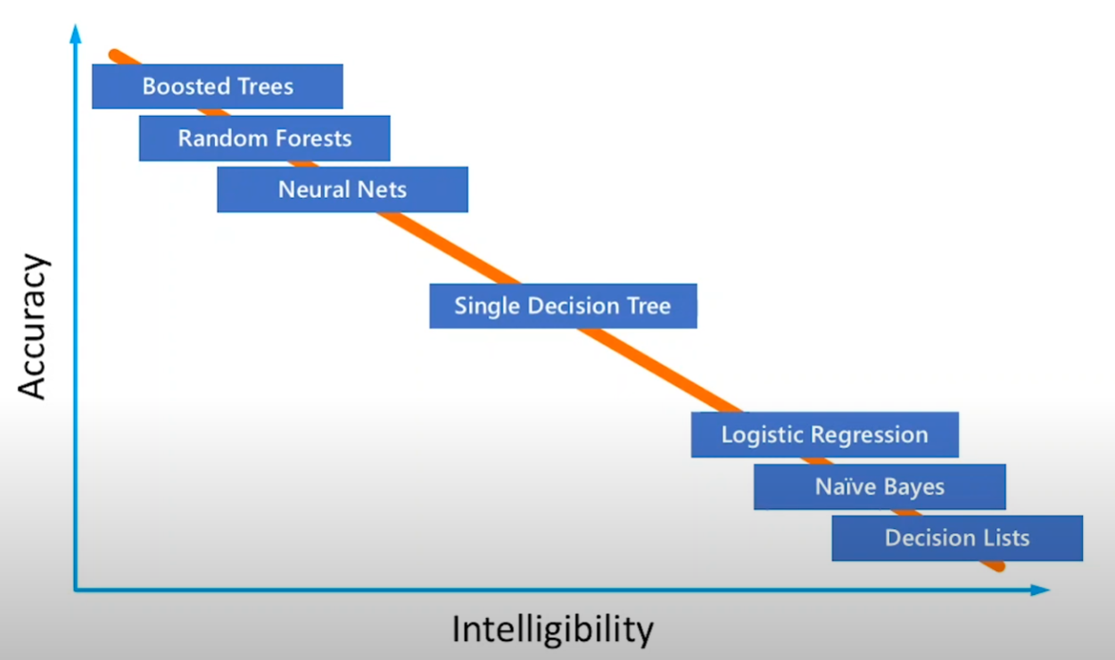
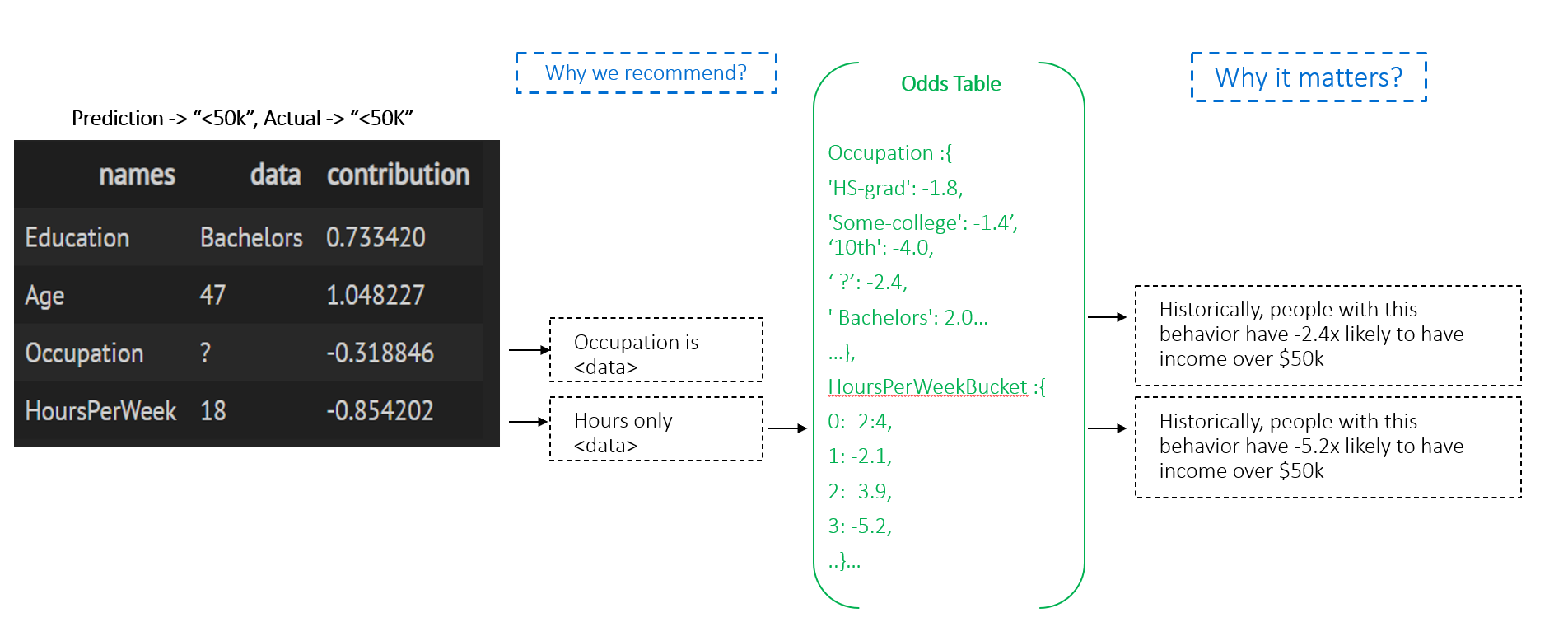
{'Education': {' HS-grad': -1.8, ' Some-college': -1.4, ' 10th': -4.0, ' Masters': 2.5, ' Assoc-voc': 1.1, ' Bachelors': 2.0, ' Assoc-acdm': 1.0, ' 1st-4th': -9.0, ' 11th': -4.7, ' 9th': -4.1, ' Doctorate': 3.1, ' Prof-school': 3.2, ' 12th': -2.9, ' 7th-8th': -3.8, ' 5th-6th': -6.2, ' Preschool': -245.4}, 'AgeBucket': {9: 1.8, 11: 1.5, 7: 1.4, 12: 1.2, 6: -1.1, 10: 1.8, 5: -2.3, 14: -1.2, 8: 1.6, 4: -20.0, 3: -100.0, 15: -1.3, 13: -1.1, 16: -2.1, 18: -2.4, 17: -245.3}, 'HoursPerWeekBucket': {8: -1.2, 9: 1.5, 12: 1.8, 3: -5.2, 7: -1.5, 6: -3.1, 5: -4.7, 10: 2.0, 4: -3.7, 14: 1.6, 2: -3.9, 13: 1.7, 11: 1.9, 15: 1.4, 1: -2.1, 0: -2.4, 19: 1.2, 16: 1.7, 17: 1.1, 18: 1.1}, 'Occupation': {' Machine-op-inspct': -1.8, ' ?': -2.4, ' Other-service': -7.1, ' Craft-repair': -1.0, ' Prof-specialty': 2.1, ' Handlers-cleaners': -3.9, ' Exec-managerial': 2.3, ' Sales': 1.1, ' Adm-clerical': -2.0, ' Transport-moving': -1.2, ' Tech-support': 1.2, ' Protective-serv': 1.4, ' Farming-fishing': -2.0, ' Priv-house-serv': -15.2, ' Armed-Forces': -1.9}}

Now using this odds table, we can generate predictions with the pre-filled template. Refer to the image below.

Fig 9. Output to human-readable text

With our explainDF data generated for row index 0 previously, we can use the above framework to convert it to text. Let us see what the output looks like -

Code
def explainPredictions(df, pred, odds_dict):
    reasons = []
    if pred == 0:
        sdf =  df.loc[df.contribution < 0, :].sort_values(['contribution']).reset_index(drop=True).copy()
    else:
        sdf =  df.loc[df.contribution > 0, :].reset_index(drop=True).copy()
    
    for idx in range(sdf.shape[0]):
        col_name = sdf.names[idx]
        data = sdf.data[idx]
        if col_name in odds_dict:
            odd_value = odds_dict[col_name][data]
        else:
            odd_value = odds_dict[col_name+'Bucket'][data//5]
            
        s1 = f"This individual have {col_name} value '{data}'." 
        s2 = f"Historically, people with this behavior have {odd_value}x likely to have income over $50k."
        reasons.append(s1+s2)
    return reasons
explainPredictions(explainDF, ebm_local.data(0)['perf']['predicted'], odds_dict)
["This individual have HoursPerWeek value '18'.Historically, people with this behavior have -5.2x likely to have income over $50k.",
 "This individual have Occupation value ' ?'.Historically, people with this behavior have -2.4x likely to have income over $50k."]

What if this was a >50k prediction?

explainPredictions(explainDF, 1, odds_dict)
["This individual have Education value ' Bachelors'.Historically, people with this behavior have 2.0x likely to have income over $50k.",
 "This individual have Age value '47'.Historically, people with this behavior have 1.8x likely to have income over $50k."]

Looks great! We can generate human-readable recommendations for both >50K and <= 50K cases. Hope this provides you with some ideas on how to implement such human-readable explanations.

Summary

In the blog, we saw the interpretability-accuracy trade-off. How Explainable Boosting Machines (EBMs) work and how they help in building models which are highly interpretable and accurate. We saw how we can use EBMs through code to generate local and global explanations and how historical odd tables and some pre-generated text can help you convert these explanations into more human-friendly text.

I hope you enjoyed reading it, and feel free to use my approach to try it out for your purposes. Also, if there is any feedback on the code or just the blog post, feel free to reach out on LinkedIn or email me at aayushmnit@gmail.com. You can also follow me on Medium and Github for future blog posts and exploration project codes I might share.

Footnotes

  1. “InterpretML: A Unified Framework for Machine Learning Interpretability” (H. Nori, S. Jenkins, P. Koch, and R. Caruana 2019)↩︎

  2. “Interpret ML - EBM documentation”↩︎

  3. Dua, D. and Graff, C. (2019). UCI Machine Learning Repository [http://archive.ics.uci.edu/ml]. Irvine, CA: University of California, School of Information and Computer Science. This dataset is licensed under a Creative Commons Attribution 4.0 International (CC BY 4.0) license.↩︎